By William J. Esposito, Doctoral Candidate and Gregory T.A. Kovacs, Professor of Electrical Engineering, Stanford University
R0.7, 5/14/14
Overview
The FFT Spectrum Visualizer takes in a signal (sound, electricity, noise) and shows the tones that make up that signal.
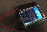
Figure 1: FFT spectrum visualizer.
For example, in a musical piece, two musical instruments could be playing tones at different frequencies. The spectrum reveals exactly what tones make up that sound.
It displays the spectrum of tones in a signal acquired with the Analog Shield and computes the spectrum using the Fast Hartley Transform (FHT) library from Open Music Labs (http://wiki.openmusiclabs.com/wiki/ArduinoFHT). The FHT function is a modified version of the Fast Fourier Transform optimized for strictly real input data [1].
The system offers touchscreen selectable log and linear scaling as well as selectable frequency span from 1kHz to 30kHz.
Hardware
The FFT Spectrum Visualizer is built around the Arduino and two shields, the Digilent Analog Shield*, and the Adafruit 2.8” TFT Touch Shield (v2), a 320x240 pixel touchscreen LCD. The Analog Shield is used for signal acquisition, and the Adafruit Touch LCD Shield is to display the spectrum.
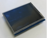
Figure 2: Adafruit touch LCD.
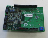
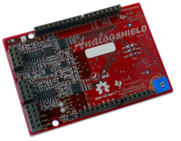
Figure 3: Analog Shield, showing space for prototyping breadboard. Protoype Analog Shield. The final shield is red.
The
Arduino UNO R3 Can be found at:
http://store.arduino.cc/
The
Adafruit RGB LCD Kit can be found at:
http://www.adafruit.com/products/1651
The Analog Shield can be found at:
http://www.digilentinc.com/analogshield
Also recommended is some sort of input. At least a headphone jack or plug (see the “Input” section). Eventually, advanced users may want to build an anti-aliasing filter as well, although this is not necessary. It is discussed in a separate section for the interested reader.
To
build the microphone input circuit, you will need:
1x LM741 Op Amp (or equivalent)
1x Electret Microphone
1x1kΩ Resistor
1x10kΩ Resistor
1x200kΩ Resistor
1x100nF Capacitor
Some solid core wire suited for breadboard use.
If you wish to use a line level input, you will also need a 3.5mm headphone jack.
Building the Demo
In order to build the Analog Shield FFT Visualizer, five nonstandard Arduino libraries are required. For a guide on Arduino libraries and how to install them, go to http://arduino.cc/en/Guide/Libraries
The libraries required for the visualizer
are.
The
Open Music Labs FHT library
http://wiki.openmusiclabs.com/wiki/ArduinoFHT
The Adafruit ILI9341 library (For the LCD )
http://github.com/adafruit/Adafruit_ILI9341
The
Adafruit GFX library (For the LCD)
http://github.com/adafruit/Adafruit-GFX-Library
The
Adafruit STMPE610 library (For Touch Functionality)
http://github.com/adafruit/Adafruit_STMPE610
The
Analog Shield library (for analog input)
http://www.github.com/wespo/analogshield
In case these libraries move in the future, the Adafruit LCD libraries are linked from the Adafruit Touch LCD Shield tutorial at
http://learn.adafruit.com/adafruit-2-8-tft-touch-shield-v2
Once these libraries are downloaded and unzipped in the Arduino/libraries folder, be sure to re-open the Arduino IDE as it will not recognize libraries added while the program is open. Once the libraries are ready, stack the LCD and Analog Shield on the Arduino Uno. Next open the “FFT_Visualizer” sketch with the Arduino IDE and upload it to the Arduino UNO. Some data will appear on screen, although the visualizer does not yet have a signal. This data represents the inherent noise in the Spectrum Visualizer and the environment.
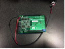
Figure 4: Headphone jack input.
Input
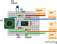
Figure 5: Microphone circuit layout.
To actually use the visualizer, some signal input is needed. Input from a signal generator is the obvious solution for an initial test, so any sort of handy sine wave generator will work. Hook the sine wave output between A0 and Ground and run. Be sure to not exceed the safe voltage of the Analog Shield, +/-5V.
A function generator is not a very satisfying test. Many hobbyists and students do not have convenient access to a good signal generator, and almost everyone will eventually want to investigate real world signals.
One option is to simply use line level (0-1.4V) audio as an input source. A standard 3.5mm (1/8”) headphone jack soldered to breadboard wire can be connected to the headers of the Analog Shield. With this, the spectrum of playing music can easily be observed. Figure 4 shows the Spectrum Visualizer with a headphone jack attached and LCD removed.
Going one step farther, one can connect a microphone to the analog shield. After all, watching the spectrum move around as a person sings a tune or whistles, is fascinating.
A fairly straightforward solution is to obtain an electret microphone[2] and an amplifier. Figures 5 and 6 show an example circuit using a commonly available electret microphone and an inexpensive LM741 Amplifier. For better performance, a higher performance amp, like an LF356 amplifier can be used . (U1 is the electret microphone).
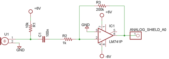
Figure 6: Electret microphone circuit schematic.
Using the Analyzer
With a signal in the analyzer, it is worth discussing how to use the analyzer itself.
The main display shows the spectrum of the signal received, which is a plot of the tones of the received signal. Increasing in frequency from left to right, the left most column reflects the power in the signal at 0Hz (DC) and the right most column the power in the signal at about 30kHz. Each column reflects a the power of a distinct frequency bin (band).
Tapping the main display (where the spectrum is displayed) will toggle the grid on and off. The grid shows the magnitude (strength) of a signal on the vertical axis and the frequency of the signal received on the horizontal axis. Toggling the grid off will allow for faster screen updates (a smoother output).
Tapping the ‘span’ button changes how wide of a frequency range the system samples. There are several steps from 1kHz to 30kHz. Switching to a smaller range means that individual frequency bins represent a smaller frequency band, but a smaller total frequency range is measured.
Finally, tapping the ‘magnitude’ button will switch between a logarithmic display and a linear output. A logarithmic output is generally more useful as it is more representative of how we perceive sounds, and makes small signals more visible.
How the Code Works
The FFT Spectrum Visualizer follows a fairly straightforward program flow. With each iteration of the main loop, it acquires an array containing 256 samples of 16-bit data from the Analog Shield at the specified sample rate. Once the array has been acquired, it passes the data to the FHT function, which transforms the time domain samples of a waveform in the array into a frequency spectrum. Finally, the resultant 16 bit spectrum is converted to an 8-bit range (on a logarithmic or linear y-axis scale) so that it can be reasonably displayed on our 240 pixel tall LCD.
Once the spectrum is ready to display, the system spends a few tens of milliseconds updating the LCD, as well as checking for touchscreen input and minor housekeeping. It then repeats the process. For slow sample rates (with a frequency span close to 1kHz) the screen update delay is a fairly small part of the overall display frame rate (a few frames per second). At high sample rates, the screen refresh time is the dominant factor and the display output appears to be continuous.
The section of code below is not meant to convey the entire code, but merely the program flow of the main loop. The entire program has many helper functions and takes up several hundred lines, not including the invoked libraries. The full code can be found at
void loop() {
while(1) { //not leaving the loop function reduces jitter
cli(); //stop all interrupts for acquisition.
if(span == 30) //fastest frequency range, no sample delay
{
for (int i = 0 ; i < FHT_N ; i++) { // save 256 samples
fht_input[i] = analog.signedRead(0); // put real data into bins
}
}
else //any other frequency span.
{
for (int i = 0 ; i < FHT_N ; i++) { // save 256 samples
fht_input[i] = analog.signedRead(0); // put real data into bins
delayMicroseconds(spanDelay); //wait to lower sample rate
}
}
//now, the fourier functions!
fht_window(); // window the data for better frequency response
fht_reorder(); // reorder the data before doing the fht
fht_run(); // process the data in the fht
if(linLog) //decide if output is going to be linear or logarithmic.
{
fht_mag_lin8(); // take the output of the fht
}
else
{
fht_mag_log(); // take the output of the fht
}
sei(); //start interrupts back up and build our display
SPI.setDataMode(SPI_MODE0); //correct SPI Mode for the LCD
if(linLog) //draw the display in the right mode
{
drawBins(fht_lin_out8); //draw the screen.
}
else
{
drawBins(fht_log_out); //draw the screen.
}
SPI.setDataMode(SPI_MODE3); // correct SPI mode for analog.read();
}
}
Anti-Aliasing Filter
To improve the analyzer, an anti-aliasing filter can be added.
The process of sampling a digital signal into the analog domain causes frequencies too high to be accurately captured by the Analog to Digital conversion to falsely reappear as lower frequencies in the digitized signal[2]. Signals seem to wrap around, or ‘bounce off’ the top of the spectrum plot.
Figure 7: Anti-aliasing filter.
The FFT spectrum visualizer can actually provide a fantastic demonstration of aliasing and the need for an anti-aliasing filter. If the FFT Visualizer is set to a 1kHz span and given an input sine wave at 500Hz (for example, using a headphone jack and an online tone generator), there will be sharp peak in the middle of the spectrum. If the input frequency is increased to 800Hz, the peak will move to the right. Above 1kHz (1000Hz) the peak would begin to move ‘backwards’ (to the left), even as the frequency continues to increase. At 1.5kHz, the peak would once again be in the center of the spectrum. At 2kHz, the peak reaches the left hand side, and then starts moving rightward again! By 2.5kHz it would once again return to the middle of the display, appearing for all intents and purposes identical to the 500Hz signal! Clearly, this is a problem.
The solution to this is an analog ‘low pass’ filter between the input signal and the input to the Analog Shield. A low pass filter is used to remove the higher frequencies before they are digitized, passing only the frequencies of interest.
In an ideal world, this filter would act like a brick wall, perfectly passing frequencies up to the highest one that the Visualizer can capture and perfectly eliminating all others. Unfortunately, such filters can’t be made in the real world, as making a sharper edge requires a more complicated filter. A truly perfect cutoff would require an infinitely large filter!
For the 30kHz sample mode, an example anti-aliasing filter design with a cutoff at 24kHz and a stop band at 40kHz has been shared with this document, as Figure 7. This filter is not perfect, as signals between 24kHz and the highest frequency bin (around 30kHz) would appear weaker than they actually are. Furthermore, signals between 30kHz and 40kHz will still appear, as if they are actually signals below 30kHz, but these tradeoffs have to be made. Ideally, one would simply not show the bins between 24 and 30kHz, but given the flexible nature of this project and the fact that it is already limited to 30kHz, those bins have been kept.
It stands to reason that if the FFT Visualizer is set to 1kHz mode, a filter with a cutoff near 1kHz should be chosen, offering similar behaviors to the 30kHz filter, but at lower frequencies. Such a design hasn’t been included here, but TI Webench (www.ti.com/webench), or many other free filter design tools can easily design such a filter.
For any active filter, the signal from outside should go into the input of the filter; output from the filter should be connected to the input (A0) of the Analog Shield. Power can be drawn from the Analog Shield’s onboard adjustable supply.
Notes
[1] Cypress semiconductor has a whitepaper explaining the differences between the FFT and FHT, it can be found at http://www.cypress.com/?docID=43614
[2] An electret microphone is a simple microphone that is fairly easy to wire up, see the Wikipedia article at http://en.wikipedia.org/wiki/Electret_microphone. Sparkfun sells a standard electret https://www.sparkfun.com/products/8635, although it is identical to one you can get at Radio Shack or any commodity electronic components store.
[3] Maxim Integrated has put together a clear article describing the need for and benefit of an anti-aliasing filter which can be found at http://www.maximintegrated.com/app-notes/index.mvp/id/928.
Disclaimer:
This code and circuit was developed by William Esposito, Ph.D. Candidate in Electrical Engineering, Stanford University, in the Kovacs/Giovangrandi Laboratory in collaboration with Texas Instruments, Incorporated. All code herein is free and open source, but is provided as-is with no warranties implied or provided. Use of this code and the associated documentation is at the user’s own risk.
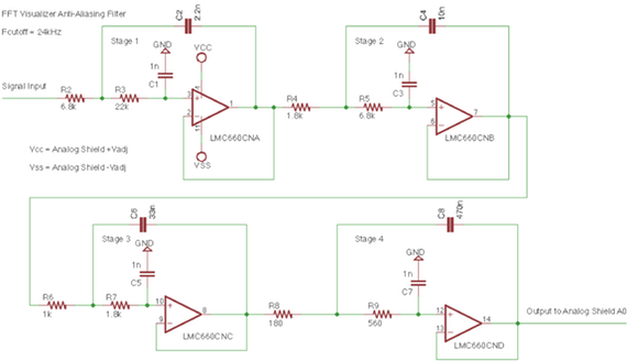 Figure 8: LPF with 24kHz Cutoff.